仓库源文，站点原文

layout: post title: GROMACS电场的使用 categories:

科 tags:
gmx math: true

2016-06-29 11:05:40

GROMACS源代码中有关电场的代码至少可追溯至3.3版本, 但由于低版本手册中没有提及, 所以很多人以为GROMACS是不支持电场的. 在GROMACS 5.x版本的手册中虽然提到了电场的选项, 但仍语焉不详, 且说明与实际代码实现不一致, 导致很多误解. 在这里, 我根据网上查阅到的资料, 以及源代码和实际测试, 对GROMACS的电场选项说明一下. 使用的GROMACS版本为5.1.2.

手册7.3.26中电场选项的说明

E-x; E-y; E-z:

如果你想在某个方向上使用电场, 在适当的E-*后输入3个数字. 第一个数字为余弦的数目, 因为只实现了单个余弦项(频率为0), 所以输入1即可; 第二个数字: 电场强度, 以V/nm为单位; 第三个数字: 余弦的相位, 你可以在这里输入任何数字, 因为频率为零的余弦没有相位.

补充说明

实际上, 这几个选项在源码中称为电场的空间部分, 也就是电场不随时间变化的部分, 即用以设定电场强度. 这里你也可以使用多个余弦项, 每个余弦项指定两个参数, 强度大小和相位. 但正如上面所说, 代码中只实现了使用一个余弦项的功能, 所以即便指定了多个余弦项, 也只有第一个起作用, 其他被忽略. 另外, 只有设定的电场强度有意义, 相位参数没有在代码中使用, 所有随意给个数字即可.

例如, 你可以使用两个余弦项, 那就指定E-x = 2 第一项电场强度任意数字第二项电场强度任意数字, 但效果与E-x = 1 电场强度任意数字是一样的. 还要注意, 第一个数字必须写为整数, 不能带小数点, 写成1.0这种会出问题.

E-xt; E-yt; E-zt:

使用这些选项你可以设置一个脉冲交变电场. 这个交变电场的形式为高斯脉冲:

$$E(t) = E_0 \exp \left[-{(t-t_0)^2 \over 2 \s^2} \right] \cos\left[\w(t-t_0)\right]$$

例如, x方向的E-x和E-xt各自有三个字段, 一共需要定义四个参数, 就像下面这样:

E-x = 1 E0 0

<del><code>E-xt = omega t0 sigma</code></del>

<del>在特殊的例子里如果 <code>sigma = 0</code>, 那么指数项将被省略, 只使用余弦项.</del>

更多的细节可参考论文Carl Caleman and David van der Spoel: Picosecond Melting of Ice by an Infrared Laser Pulse - A Simulation Study Angew. Chem. Intl. Ed. 47 pp. 14 17-1420 (2008)。

补充说明

这几个选项称为电场的时间部分, 也就是电场随时间变化的部分, 不包含空间强度部分的信息. 手册中的说明有误, 错误部分已经标识删除线.

在这里你可以选择使用单个余弦变化的电场, 或是高斯脉冲交变电场. 但选项参数的设置有讲究, 且高斯脉冲电场的sigma参数不能为0, 否则运行出错.

与E-x等选项一样, E-xt等选项的参数设置格式中, 第一个数字也是余弦项的数目, 后面跟着每个余弦项的频率omega和相位phi, 但源码中没有使用phi, 所以只有设定的omega有意义, phi可以随意给个数字.

使用高斯脉冲电场时, E-xt等选项的第一个参数必须为3, 且后面跟着6个数字, 分别是omega 任意数字 t0 任意数字 sigma 任意数字.

使用余弦电场时, Ex-t等选项的第一个参数不为3即可, 但仍然只有第一项起作用, 所以使用1 omega 任意数字即可.

源代码中的电场部分

GROMACS中电场的实现代码位于.\gromacs-5.1.2\src\gromacs\mdlib\sim_util.cpp的calc_f_el函数,

<table class="highlighttable"><th colspan="2" style="text-align:left">c</th><tr><td><div class="linenodiv" style="background-color: #f0f0f0; padding-right: 10px"><pre style="line-height: 125%"> 1 2 3 4 5 6 7 8 9 10 11 12 13 14 15 16 17 18 19 20 21 22 23 24 25 26 27 28 29 30 31 32 33 34 35 36 37 38 39 40 41 42 43 44 45 46 47 48 49 50 51 52 53 54 55 56 57 58 59 60 61 62 63 64 65 66 67</pre></div></td><td class="code"><div class="highlight" style="background: #f8f8f8"><pre style="line-height: 125%">/* * calc_f_el calculates forces due to an electric field. * * force is kJ mol^-1 nm^-1 = e * kJ mol^-1 nm^-1 / e * * Et[] contains the parameters for the time dependent * part of the field. * Ex[] contains the parameters for * the spatial dependent part of the field. * The function should return the energy due to the electric field * (if any) but for now returns 0. * * WARNING: * There can be problems with the virial. * Since the field is not self-consistent this is unavoidable. * For neutral molecules the virial is correct within this approximation. * For neutral systems with many charged molecules the error is small. * But for systems with a net charge or a few charged molecules * the error can be significant when the field is high. * Solution: implement a self-consistent electric field into PME. */ static void calc_f_el(FILE *fp, int start, int homenr, real charge[], rvec f[], t_cosines Ex[], t_cosines Et[], double t) { rvec Ext; real t0; int i, m; for (m = 0; (m < DIM); m++) { if (Et[m].n > 0) { if (Et[m].n == 3) { t0 = Et[m].a[1]; Ext[m] = cos(Et[m].a[0]*(t-t0))*exp(-sqr(t-t0)/(2.0*sqr(Et[m].a[2]))); } else { Ext[m] = cos(Et[m].a[0]*t); } } else { Ext[m] = 1.0; } if (Ex[m].n > 0) { /* Convert the field strength from V/nm to MD-units */ Ext[m] *= Ex[m].a[0]*FIELDFAC; for (i = start; (i < start+homenr); i++) { f[i][m] += charge[i]*Ext[m]; } } else { Ext[m] = 0; } } if (fp != NULL) { fprintf(fp, "%10g %10g %10g %10g #FIELD\n", t, Ext[XX]/FIELDFAC, Ext[YY]/FIELDFAC, Ext[ZZ]/FIELDFAC); } } </pre></div> </td></tr></table>

可以看到, 函数calc_f_el中传入的Ex[]和Et[]的数据类型都是t_cosines. 这种数据类型的定义于.\gromacs-5.1.2\src\gromacs\legacyheaders\types\inputrec.h:

<table class="highlighttable"><th colspan="2" style="text-align:left">c</th><tr><td><div class="linenodiv" style="background-color: #f0f0f0; padding-right: 10px"><pre style="line-height: 125%"> 1 2 3 4 5 6 7 8 9 10 11 12</pre></div></td><td class="code"><div class="highlight" style="background: #f8f8f8"><pre style="line-height: 125%">typedef struct { int n; /* Number of terms */ real *a; /* Coeffients (V / nm ) */ real *phi; /* Phase angles */ } t_cosines; typedef struct { real E0; /* Field strength (V/nm) */ real omega; /* Frequency (1/ps) */ real t0; /* Centre of the Gaussian pulse (ps) */ real sigma; /* Width of the Gaussian pulse (FWHM) (ps) */ } t_efield; </pre></div> </td></tr></table>

在这里我们还可以看到, 虽然定义了高斯脉冲电场使用的数据类型_efield, 但它没有传入函数calc_f_el, 所以没有办法直接使用.

如果你需要实现特殊的电场形式, 修改calc_f_el函数即可, 且可以像目前实现高斯脉冲电场的方法一样, 重用传入的参数.

<code>mdrun</code>时查看电场信息

mdrun运行模拟后, 输出的.log文件中会给出设定的电场信息, 类似于

E-x:
   n = 2
     a = 1.000000e+001 2.000000e+001
     phi = 1.000000e+001 3.000000e+001
E-xt:
   n = 3
     a = 1.000000e+003 1.000000e-001 1.000000e-002
     phi = 0.000000e+000 0.000000e+000 0.000000e+000
E-y:
   n = 0
E-yt:
   n = 0
E-z:
   n = 0
E-zt:
   n = 0

你可以从这里看到自己设定的值是否正确读入了.

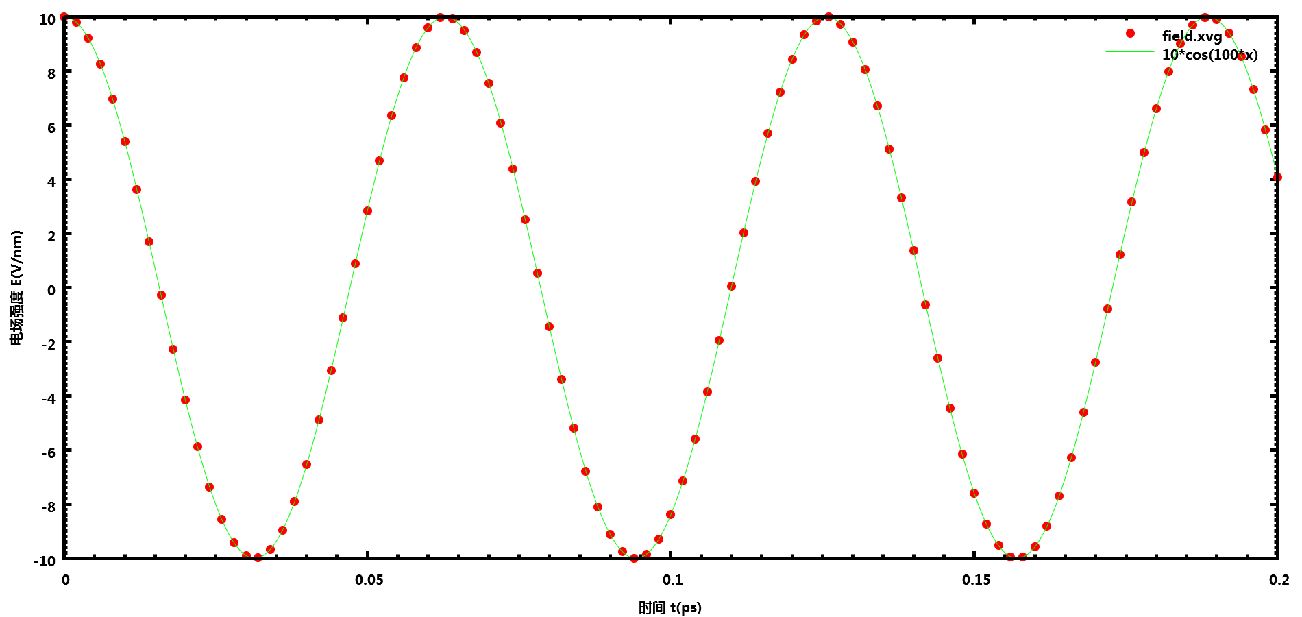
mdrun运行时有一个选项-field, 可以指定一个.xvg文件, 里面记录每个时间步的电场大小, 默认输出文件为field.xvg. 利用这个文件你可以查看所加的电场是否正确.

余弦电场

在.mdp中的设置强度为10 V/nm, 频率为100 ps-1(即100 THz)的余弦电场

E-x              = 1 10 0
E-xt             = 1 100 0

GROMACS输出的数据与设置完全一致

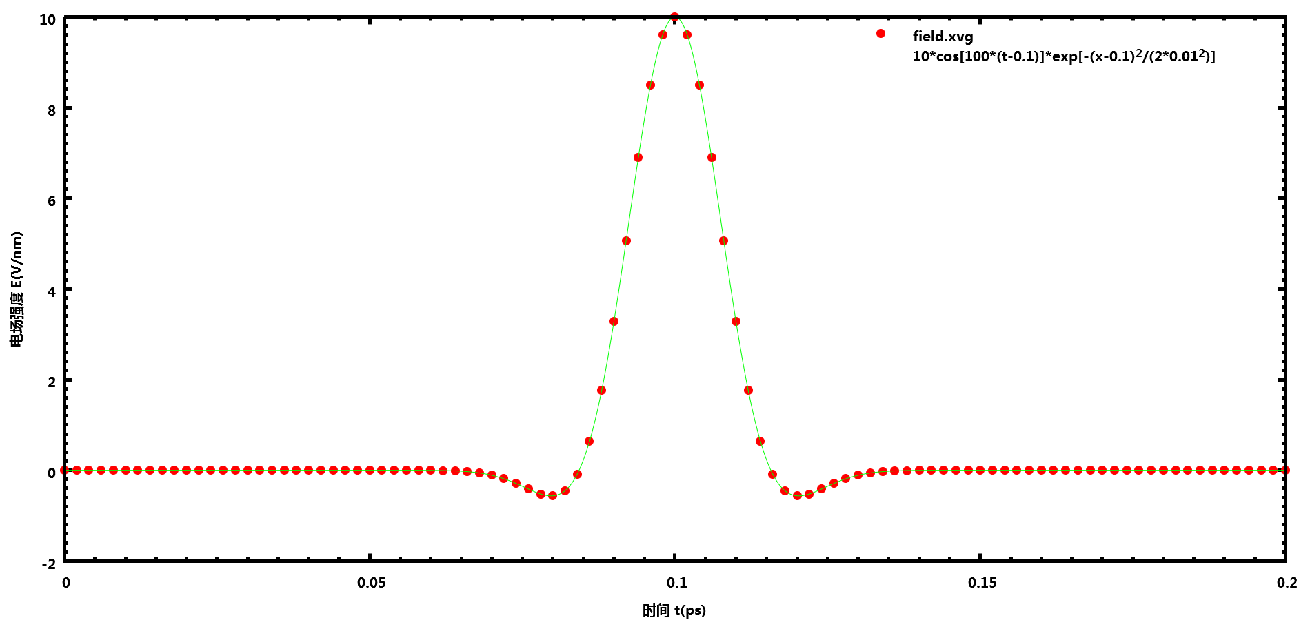
高斯脉冲电场

在.mdp中的设置强度为10 V/nm, 频率为100 ps-1(即100 THz), 脉冲中心0.1 ps, 方差0.01 ps的高斯脉冲电场

E-x              = 1 10 0
E-xt             = 3 100 0 .1 0 .01 0

GROMACS输出的数据与设置完全一致

使用电场的示例

研究电场对体系的影响时, 最好先使用NVE系综进行测试, 看看.mdp中的选项设置在不加电场时能否保证能量守恒. 严格的能量守恒是很难做到的, 只要在关心的时间尺度内能量守恒即可, 也可以根据能量漂移的速率来决定, 大致小于相应温度下的平动能就能接受. 能量守恒测试通过后, 再打开电场选项, 看电场对体系总能量的影响. 成品模拟时一般是使用NVT或NPT的.

下面测试下GROMACS自带的spc216.gro水盒子NVE系综下不同电场的影响, 电场设置与上面的相同.

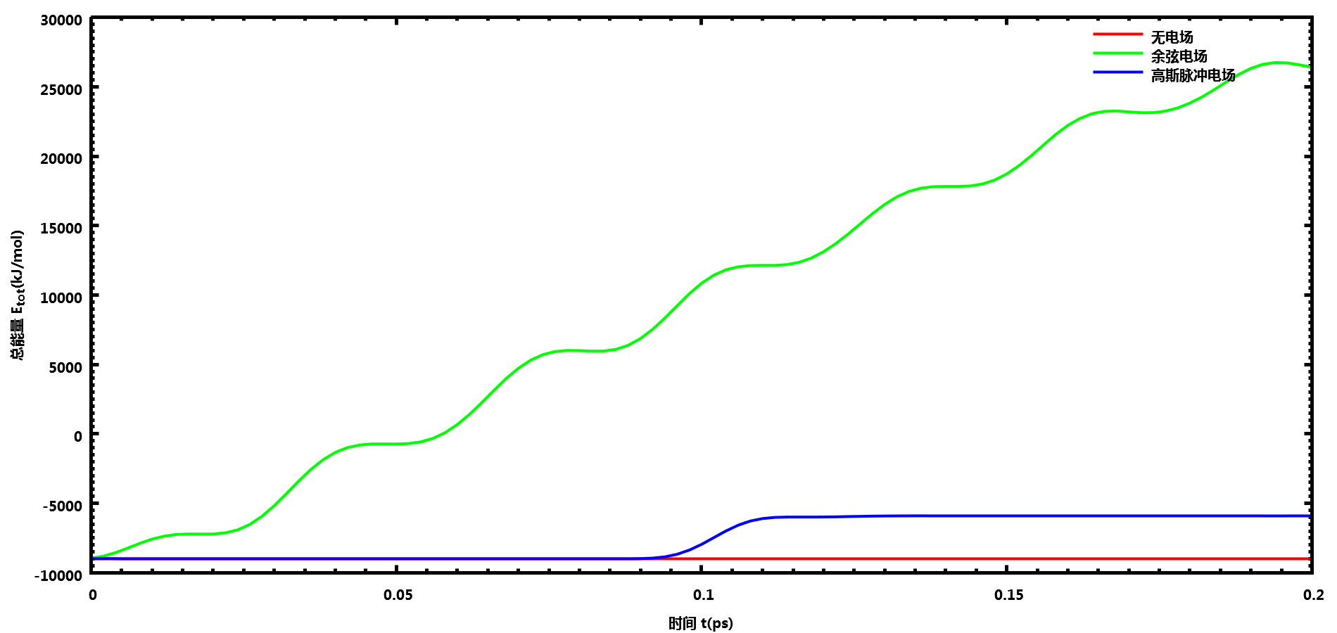
可以看到加了电场后, 体系总能量会增大很多. 你可以下载所用的文件, 自己进行测试.

参考资料

2017-02-20 14:29:52 hjx 非常不错，学习了。感谢李老师。